Today, I’ll add an entry to my occasional reviews of interesting academic papers. The paper: "Price Level and Inflation Dynamics in Heterogeneous Agent…
One of the many reasons I am excited about this paper is that it unites fiscal theory of the price level with heterogeneous agent economics. And it shows how heterogeneity matters. There has been a lot of work on "heterogeneous agent new-Keynesian" models (HANK). This paper inaugurates heterogeneous agent fiscal theory models. Let's call them HAFT.
The paper has a beautifully stripped down model. Prices are flexible, and the price level is set by fiscal theory. People face uninsurable income shocks, however, and a borrowing limit. So they save an extra amount in order to self-insure against bad times. Government bonds are the only asset in the model, so this extra saving pushes down the interest rate, discount rate, and government service debt cost. The model has a time-zero shock and then no aggregate uncertainty.
This is exactly the right place to start. In the end, of course, we want fiscal theory, heterogeneous agents, and sticky prices to add inflation dynamics. And on top of that, whatever DSGE smorgasbord is important to the issues at hand; production side, international trade, multiple real assets, financial fractions, and more. But the genius of a great paper is to start with the minimal model.
Part II effects of fiscal shocks.
I am most excited by part II, the effects of fiscal shocks. This goes straight to important policy questions.
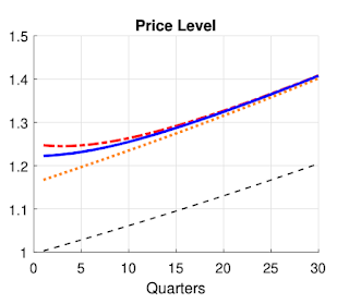
Note: This figure plots impulse responses to a targeted and untargeted helicopter drop, aggregated at the quarterly frequency. The helicopter drop is a one-time issuance of 16% of total government nominal debt outstanding at t = 0. Only households in the bottom 60% of the wealth distribution receive the issuance in the targeted experiment (dashed red line). The orange line plots dynamics in the representative agent (RA) model. The dashed black line plots the initial steady state. Source: Kaplan et al. Figure 7
At time 0, the government drops $5 trillion of extra debt on people, with no plans to pay it back. The interest rate does not change. What happens? In the representative agent economy, the price level jumps, just enough to inflate away outstanding debt by $5 trillion.
(In this simulation, inflation subsequent to the price level jump is just set by the central bank, via an interest rate target. So the rising price level line of the representative agent (orange) benchmark is not that interesting. It's not a conventional impulse response showing the change after the shock; it's the actual path after the shock. The difference between colored heterogeneous agent lines and the orange representative agent line is the important part.)
Punchline: In the heterogeneous agent economies, the price level jumps a good deal more. And if transfers are targeted to the bottom of the wealth distribution, the price level jumps more still. It matters who gets the money.
This is the first step on an important policy question. Why was the 2020-2021 stimulus so much more inflationary than, say 2008? I have a lot of stories ("fiscal histories," FTPL), one of which is a vague sense that printing money and sending people checks has more effect than borrowing in treasury markets and spending the results. This graph makes that sense precise. Sending people checks, especially people who are on the edge, does generate more inflation.
In the end, whether government debt is inflationary or not comes down to whether people treat the asset as a good savings vehicle, and hang on to it, or try to spend it, thereby driving up prices. Sending checks to people likely to spend it gives more inflation.
As you can see, the model also introduces some dynamics, where in this simple setup (flexible prices) the RA model just gives a price level jump. To understand those dynamics, and more intuition of the model, look at the response of real debt and the real interest rate
The greater inflation means that the same increase in nominal debt is a lesser increase in real debt. Now, the crucial feature of the model steps in: due to self-insurance, there is essentially a liquidity value of debt. If you have less debt, the marginal value of higher; people bid down the real interest rate in an attempt to get more debt. But the higher real rate means the real value of debt rises, and as the debt rises, the real interest rate falls.
To understand why this is the equilibrium, it's worth looking at the debt accumulation equation, [ frac{db}{dt} = r_t (b_t; g_t) b_t - s_t. ](b_t) is the real value of nominal debt, (r_t=i_t-pi_t) is the real interest rate, and (s_t) is the real primary surplus. Higher real rates (debt service costs) raise debt. Higher primary surpluses pay down debt. Crucially -- the whole point of the paper -- the interest rate depends on how much debt is outstanding and on the distribution of wealth (g_t). ((g_t) is a whole distribution.) More debt means a higher interest rate. More debt does a better job of satisfying self-insurance motives. Then the marginal value of debt is lower, so people don't try to save as much, and the interest rate rises. It works a lot like money demand,
Now, if the transfer were proportional to current wealth, nothing would change, the price level would jump just like the RA (orange) line. But it isn't; in both cases more-constrained people get more money. The liquidity constraints are less binding, they're willing to save more. For given aggregate debt the real interest rate will rise. So the orange line with no change in real debt is no longer a steady state. We must have, initially (db/dt>0.) Once debt rises and the distribution of wealth mixes, we go back to the old steady state, so real debt rises less initially, so it can continue to rise. And to do that, we need a larger price level jump. Whew. (I hope I got that right. Intuition is hard!)
In a previous post on heterogeneous agent models, I asked whether HA matters for aggregates, or whether it is just about distributional consequences of unchanged aggregate dynamics. Here is a great example in which HA matters for aggregates, both for the size and for the dynamics of the effects.
Here's a second cool simulation. What if, rather than a lump-sum helicopter drop with no change in surpluses, the government just starts running permanent primary deficits?
Note: Impulse response to a permanent expansion in primary deficits. The dotted orange line shows the effects of a reduction in surplus in the Representative Agent model. The blue line labelled “Lump Sum” illustrates the dynamics following an expansion of lump sum transfers. The dashed red line labelled “Tax Rate” plots dynamics following a tax cut. The orange line plots dynamics in the representative agent (RA) model. The dashed black line plots the initial steady state. Source: Kaplan et. al. Figure 8.
In the RA model, a decline in surpluses is exactly the same thing as a rise in debt. You get the initial price jump, and then the same inflation following the interest rate target. Not so the HA models! Perpetual deficits are different from a jump in debt with no change in deficit.
Again, real debt and the real rate help to understand the intuition. The real amount of debt is permanently lower. That means people are more starved for buffer stock assets, and bid down the real interest rate. The nominal rate is fixed, by assumption in this simulation, so a lower real rate means more inflation.
For policy, this is an important result. With flexible prices, RA fiscal theory only gives a one-time price level jump in response to unexpected fiscal shocks. It does not give steady inflation in response to steady deficits. Here we do have steady inflation in response to steady deficits! It also shows an instance of the general "discount rates matter" theorem. Granted, here, the central bank could lower inflation by just lowering the nominal rate target but we know that's not so easy when we add realisms to the model.
To see just why this is the equilibrium, and why surpluses are different than debt, again go back to the debt accumulation equation, [ frac{db}{dt} = r_t (b_t, g_t) b_t - s_t. ] In the RA model, the price level jumps so that (b_t) jumps down, and then with smaller (s_t), (r b_t - s_t) is unchanged with a constant (r). But in the HA model, the lower value of (b) means less liquidity value of debt, and people try to save, bidding down the interest rate. We need to work down the debt demand curve, driving down the real interest costs (r) until they partially pay for some of the deficits. There is a sense in which "financial repression" (artificially low interest rates) via perpetual inflation help to pay for perpetual deficits. Wow!
Part I r<g
The first theory part of the paper is also interesting. (Though these are really two papers stapled together, since as I see it the theory in the first part is not at all necessary for the simulations.) Here, Kaplan, Nikolakoudis and Violante take on the r<g question clearly. No, r<g does not doom fiscal theory! I was so enthused by this that I wrote up a little note "fiscal theory with negative interest rates" here. Detailed algebra of my points below are in that note, (An essay r<g and also a r<g chapter in FTPL explains the related issue, why it's a mistake to use averages from our real economy to calibrate perfect foresight models. Yes, we can observe (E(r)<E(g)) yet present values converge.)
I'll give the basic idea here. To keep it simple, think about the question what happens with a negative real interest rate (r<0), a constant surplus (s) in an economy with no growth, and perfect foresight. You might think we're in trouble: [b_t = frac{B_t}{P_t} = int e^{-rtau} s dtau = frac{s}{r}.]A negative interest rate makes present values blow up, no? Well, what about a permanently negative surplus (s<0) financed by a permanently negative interest cost (r<0)? That sounds fine in flow terms, but it's really weird as a present value, no?
Yes, it is weird. Debt accumulates at [frac{db_t}{dt} = r_t b_t - s_t.] If (r>0), (s>0), then the real value of debt is generically explosive for any initial debt but (b_0=s/r). Because of the transversality condition ruling out real explosions, the initial price level jumps so (b_0=B_0/P_0=s/r). But if (r<0), (s<0), then debt is stable. For any (b_0), debt converges, the transversality condition is satisfied. We lose fiscal price level determination. No, you can't take a present value of a negative cashflow stream with a negative discount rate and get a sensible present value.
But (r) is not constant. The more debt, the higher the interest rate. So [frac{db_t}{dt} = r(b_t) b_t - s_t.] Linearizing around the steady state (b=s/r), [frac{db_t}{dt} = left[r_t + frac{dr(b_t)}{db}right]b_t - s.] So even if (r<0), if more debt raises the interest rate enough, if (dr(b)/db) is large enough, dynamics are locally and it turns out globally unstable even with (r<0). Fiscal theory still works!
You can work out an easy example with bonds in utility, (int e^{-rho t}[u(c_t) + theta v(b_t)]dt), and simplifying further log utility (u(c) + theta log(b)). In this case (r = rho - theta v'(b) = rho - theta/b) (see the note for derivation), so debt evolves as [frac{db}{dt} = left[rho - frac{theta}{b_t}right]b_t - s = rho b_t - theta - s.]Now the (r<0) part still gives stable dynamics and multiple equilibria. But if (theta>-s), then dynamics are again explosive for all but (b=s/r) and fiscal theory works anyway.
This is a powerful result. We usually think that in perfect foresight models, (r>g), (r>0) here, and consequently positive vs negative primary surpluses (s>0) vs. (s<0) is an important dividing line. I don't know how many fiscal theory critiques I have heard that say a) it doesn't work because r<g so present values explode b) it doesn't work because primary surpluses are always slightly negative.
This is all wrong. The analysis, as in this example, shows is that fiscal theory can work fine, and doesn't even notice, a transition from (r>0) to (r<0), from (s>0) to (s<0). Financing a steady small negative primary surplus with a steady small negative interest rate, or (r<g) is seamless.
The crucial question in this example is (s<-theta). At this boundary, there is no equilibrium any more. You can finance only so much primary deficit by financial repression, i.e. squeezing down the amount of debt so its liquidity value is high, pushing down the interest costs of debt.
The paper staples these two exercises together, and calibrates the above simulations to (s<0) and (r<g). But I bet they would look almost exactly the same with (s>0) and (r>g). (r<g) is not essential to the fiscal simulations.
The paper analyzes self-insurance against idiosyncratic shocks as the cause of a liquidity value of debt. That's interesting, and allows the authors to calibrate the liquidity value against microeconomic observations on just how much people suffer such shocks and want to insure against them. The Part I simulations are just that, heterogeneous agents in action. But this theoretical point is much broader, and applies to any economic force that pushes up the real interest rate as the volume of debt rises. Bonds in utility, here and in the paper's appendix, work. They are a common stand in for the usefulness of government bonds in financial transactions. And in that case, it's easier to extend the analysis to a capital stock, real estate, foreign borrowing and lending, gold bars, crypto, and other means of self-insuring against shocks. Standard ``crowding out'' stories by which higher debt raises interest rates work. (Blachard's r<g work has a lot of such stories.) The ``segmented markets'' stories underlying faith in QE give a rising b(r). So the general principle is robust to many different kinds of models.
My note explores one issue the paper does not, and it's an important one in asset pricing. OK, I see how dynamics are locally unstable, but how do you take a present value when r<0? If we write the steady state [b_t = int_{tau=0}^infty e^{-r tau}s dtau = int_{tau=0}^T e^{-r tau}s dtau + e^{-rT}b_{t+T}= (1-e^{-rT})frac{s}{r} + e^{-rT}b,]and with (r<0) and (s<0), the integral and final term of the present value formula each explode to infinity. It seems you really can't discount with a negative rate.
The answer is: don't integrate forward [frac{db_t}{dt}=r b_t - s ]to the nonsense [ b_t = int e^{-r tau} s dtau.]Instead, integrate forward [frac{db_t}{dt} = rho b_t - theta - s]to [b_t = int e^{-rho tau} (s + theta)dt = int e^{-rho tau} frac{u'(c_t+tau)}{u'(c_t)}(s + theta)dt.]In the last equation I put consumption ((c_t=1) in the model) for clarity.
Discount the flow value of liquidity benefits at the consumer's intertemporal marginal rate of substitution. Do not use liquidity to produce an altered discount rate.
This is another deep, and frequently violated point. Our discount factor tricks do not work in infinite-horizon models. (1=E(R_{t+1}^{-1}R_{t+1})) works just as well as (1 = Eleft[beta u'(c_{t+1})/u'(c_t)right] r_{t+1}) in a finite horizon model, but you can't always use (m_{t+1}=R_{t+1}^{-1}) in infinite period models. The integrals blow up, as in the example.
This is a good thesis topic for a theoretically minded researcher. It's something about Hilbert spaces. Though I wrote the discount factor book, I don't know how to extend discount factor tricks to infinite periods. As far as I can tell, nobody else does either. It's not in Duffie's book.
In the meantime, if you use discount factor tricks like affine models -- anything but the proper SDF -- to discount an infinite cashflow, and you find "puzzles," and "bubbles," you're on thin ice. There are lots of papers making this mistake.
A minor criticism: The paper doesn't show nuts and bolts of how to calculate a HAFT model, even in the simplest example. Note by contrast how trivial it is to calculate a bonds in utility model that gets most of the same results. Give us a recipe book for calculating textbook examples, please!
Obviously this is a first step. As FTPL quickly adds sticky prices to get reasonable inflation dynamics, so should HAFT. For FTPL (or FTMP, fiscal theory of monetary policy; i.e. adding interest rate targets), adding sticky prices made the story much more realistic: We get a year or two of steady inflation eating away at bond values, rather than a price level jump. I can't wait to see HAFT with sticky prices. For all the other requests for generalization: you just found your thesis topic.
Over the last few years, digital currencies and gold have become decent barometers of speculative investor appetite. Such isn’t surprising given the evolution…
Over the last few years, digital currencies and gold have become decent barometers of speculative investor appetite. Such isn’t surprising given the evolution of the market into a “casino” following the pandemic, where retail traders have increased their speculative appetites.
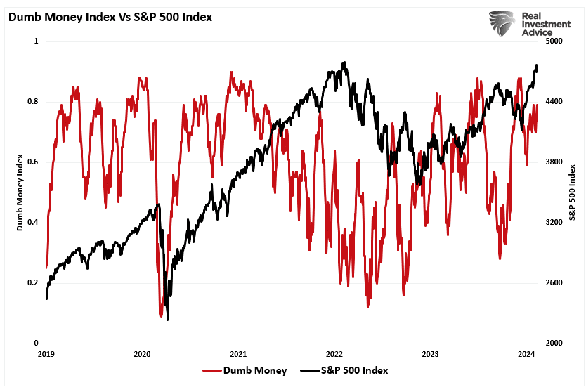
“Such is unsurprising, given that retail investors often fall victim to the psychological behavior of the “fear of missing out.” The chart below shows the “dumb money index” versus the S&P 500. Once again, retail investors are very long equities relative to the institutional players ascribed to being the “smart money.””
“The difference between “smart” and “dumb money” investors shows that, more often than not, the “dumb money” invests near market tops and sells near market bottoms.”
That enthusiasm has increased sharply since last November as stocks surged in hopes that the Federal Reserve would cut interest rates. As noted by Sentiment Trader:
“Over the past 18 weeks, the straight-up rally has moved us to an interesting juncture in the Sentiment Cycle. For the past few weeks, the S&P 500 has demonstrated a high positive correlation to the ‘Enthusiasm’ part of the cycle and a highly negative correlation to the ‘Panic’ phase.”
That frenzy to chase the markets, driven by the psychological bias of the “fear of missing out,” has permeated the entirety of the market. As noted in “This Is Nuts:”
“Since then, the entire market has surged higher following last week’s earnings report from Nvidia (NVDA). The reason I say “this is nuts” is the assumption that all companies were going to grow earnings and revenue at Nvidia’s rate. There is little doubt about Nvidia’s earnings and revenue growth rates. However, to maintain that growth pace indefinitely, particularly at 32x price-to-sales, means others like AMD and Intel must lose market share.”
Of course, it is not just a speculative frenzy in the markets for stocks, specifically anything related to “artificial intelligence,” but that exuberance has spilled over into gold and cryptocurrencies.
Birds Of A Feather
There are a couple of ways to measure exuberance in the assets. While sentiment measures examine the broad market, technical indicators can reflect exuberance on individual asset levels. However, before we get to our charts, we need a brief explanation of statistics, specifically, standard deviation.
“Like a rubber band that has been stretched too far – it must be relaxed in order to be stretched again. This is exactly the same for stock prices that are anchored to their moving averages. Trends that get overextended in one direction, or another, always return to their long-term average. Even during a strong uptrend or strong downtrend, prices often move back (revert) to a long-term moving average.”
The idea of “stretching the rubber band” can be measured in several ways, but I will limit our discussion this week to Standard Deviation and measuring deviation with “Bollinger Bands.”
“Standard Deviation” is defined as:
“A measure of the dispersion of a set of data from its mean. The more spread apart the data, the higher the deviation. Standard deviation is calculated as the square root of the variance.”
In plain English,this meansthat the further away from the average that an event occurs, the more unlikely it becomes. As shown below, out of 1000 occurrences, only three will fall outside the area of 3 standard deviations. 95.4% of the time, events will occur within two standard deviations.
A second measure of “exuberance” is “relative strength.”
“In technical analysis, the relative strength index (RSI) is a momentum indicator that measures the magnitude of recent price changes to evaluate overbought or oversold conditions in the price of a stock or other asset. The RSI is displayed as an oscillator (a line graph that moves between two extremes) and can read from 0 to 100.
Traditional interpretation and usage of the RSI are that values of 70 or above indicate that a security is becoming overbought or overvalued and may be primed for a trend reversal or corrective pullback in price. An RSI reading of 30 or below indicates an oversold or undervalued condition.” – Investopedia
With those two measures, let’s look at Nvidia (NVDA), the poster child of speculative momentum trading in the markets. Nvidia trades more than 3 standard deviations above its moving average, and its RSI is 81. The last time this occurred was in July of 2023 when Nvidia consolidated and corrected prices through November.
Interestingly, gold also trades well into 3 standard deviation territory with an RSI reading of 75. Given that gold is supposed to be a “safe haven” or “risk off” asset, it is instead getting swept up in the current market exuberance.
The same is seen with digital currencies. Given the recent approval of spot, Bitcoin exchange-traded funds (ETFs), the panic bid to buy Bitcoin has pushed the price well into 3 standard deviation territory with an RSI of 73.
In other words, the stock market frenzy to “buy anything that is going up” has spread from just a handful of stocks related to artificial intelligence to gold and digital currencies.
It’s All Relative
We can see the correlation between stock market exuberance and gold and digital currency, which has risen since 2015 but accelerated following the post-pandemic, stimulus-fueled market frenzy. Since the market, gold and cryptocurrencies, or Bitcoin for our purposes, have disparate prices, we have rebased the performance to 100 in 2015.
Gold was supposed to be an inflation hedge. Yet, in 2022, gold prices fell as the market declined and inflation surged to 9%. However, as inflation has fallen and the stock market surged, so has gold. Notably, since 2015, gold and the market have moved in a more correlated pattern, which has reduced the hedging effect of gold in portfolios. In other words, during the subsequent market decline, gold will likely track stocks lower, failing to provide its “wealth preservation” status for investors.
The same goes for cryptocurrencies. Bitcoin is substantially more volatile than gold and tends to ebb and flow with the overall market. As sentiment surges in the S&P 500, Bitcoin and other cryptocurrencies follow suit as speculative appetites increase. Unfortunately, for individuals once again piling into Bitcoin to chase rising prices, if, or when, the market corrects, the decline in cryptocurrencies will likely substantially outpace the decline in market-based equities. This is particularly the case as Wall Street can now short the spot-Bitcoin ETFs, creating additional selling pressure on Bitcoin.
Just for added measure, here is Bitcoin versus gold.
Not A Recommendation
There are many narratives surrounding the markets, digital currency, and gold. However, in today’s market, more than in previous years, all assets are getting swept up into the investor-feeding frenzy.
Sure, this time could be different. I am only making an observation and not an investment recommendation.
However, from a portfolio management perspective, it will likely pay to remain attentive to the correlated risk between asset classes. If some event causes a reversal in bullish exuberance, cash and bonds may be the only place to hide.
BUFFALO, NY- March 11, 2024 – Impact Journals publishes scholarly journals in the biomedical sciences with a focus on all areas of cancer and aging research. Aging is one of the most prominent journals published by Impact Journals.
Credit: Impact Journals
BUFFALO, NY- March 11, 2024 – Impact Journals publishes scholarly journals in the biomedical sciences with a focus on all areas of cancer and aging research. Aging is one of the most prominent journals published by Impact Journals.
Impact Journals will be participating as an exhibitor at the American Association for Cancer Research (AACR) Annual Meeting 2024 from April 5-10 at the San Diego Convention Center in San Diego, California. This year, the AACR meeting theme is “Inspiring Science • Fueling Progress • Revolutionizing Care.”
Visit booth #4159 at the AACR Annual Meeting 2024 to connect with members of the Agingteam.
About Aging-US:
Agingpublishes research papers in all fields of aging research including but not limited, aging from yeast to mammals, cellular senescence, age-related diseases such as cancer and Alzheimer’s diseases and their prevention and treatment, anti-aging strategies and drug development and especially the role of signal transduction pathways such as mTOR in aging and potential approaches to modulate these signaling pathways to extend lifespan. The journal aims to promote treatment of age-related diseases by slowing down aging, validation of anti-aging drugs by treating age-related diseases, prevention of cancer by inhibiting aging. Cancer and COVID-19 are age-related diseases.
Agingis indexed and archived byPubMed/Medline (abbreviated as “Aging (Albany NY)”), PubMed Central, Web of Science: Science Citation Index Expanded (abbreviated as “Aging‐US” and listed in the Cell Biology and Geriatrics & Gerontology categories), Scopus (abbreviated as “Aging” and listed in the Cell Biology and Aging categories), Biological Abstracts, BIOSIS Previews, EMBASE, META (Chan Zuckerberg Initiative) (2018-2022), and Dimensions (Digital Science).
Please visit our website at www.Aging-US.com and connect with us:
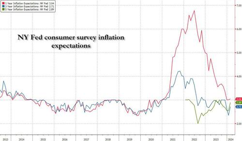
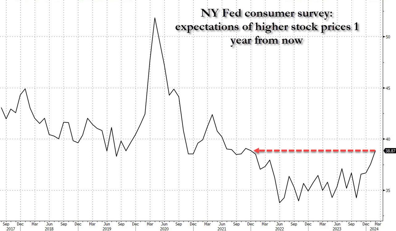
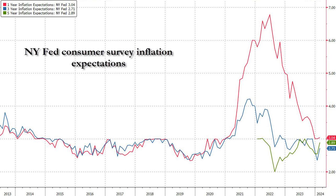
NY Fed Finds Medium, Long-Term Inflation Expectations Jump Amid Surge In Stock Market Optimism
One month after the inflation outlook tracked by the NY Fed Consumer Survey extended their late 2023 slide, with 3Y inflation expectations in January sliding to a record low 2.4% (from 2.6% in December), even as 1 and 5Y inflation forecasts remained flat, moments ago the NY Fed reported that in February there was a sharp rebound in longer-term inflation expectations, rising to 2.7% from 2.4% at the three-year ahead horizon, and jumping to 2.9% from 2.5% at the five-year ahead horizon, while the 1Y inflation outlook was flat for the 3rd month in a row, stuck at 3.0%.
The increases in both the three-year ahead and five-year ahead measures were most pronounced for respondents with at most high school degrees (in other words, the "really smart folks" are expecting deflation soon). The survey’s measure of disagreement across respondents (the difference between the 75th and 25th percentile of inflation expectations) decreased at all horizons, while the median inflation uncertainty—or the uncertainty expressed regarding future inflation outcomes—declined at the one- and three-year ahead horizons and remained unchanged at the five-year ahead horizon.
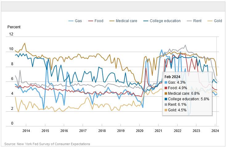
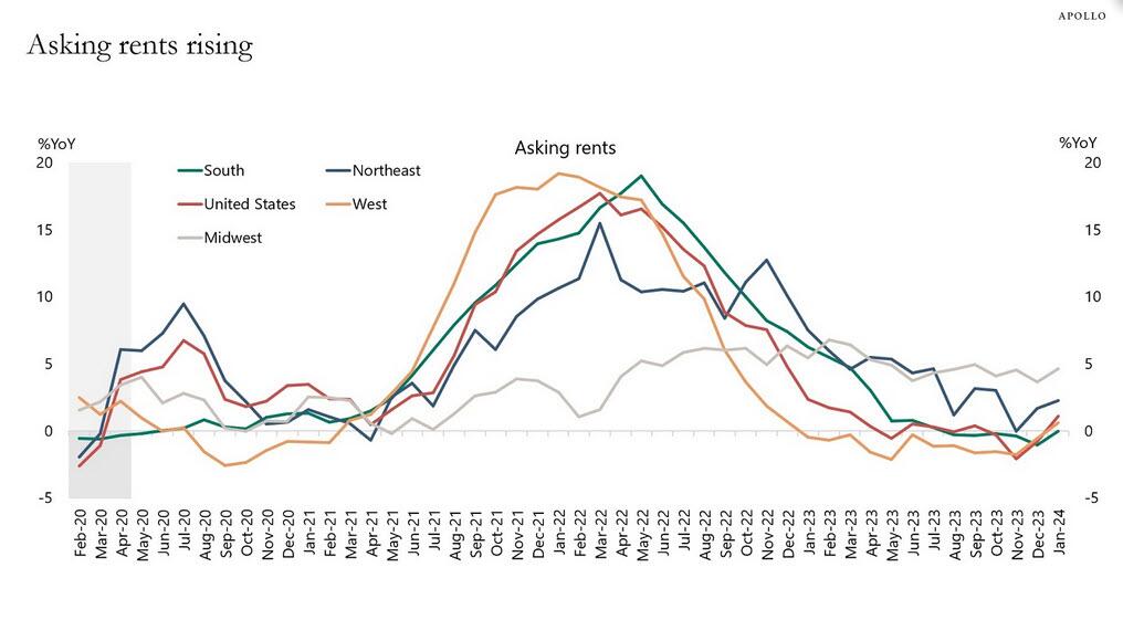
Going down the survey, we find that the median year-ahead expected price changes increased by 0.1 percentage point to 4.3% for gas; decreased by 1.8 percentage points to 6.8% for the cost of medical care (its lowest reading since September 2020); decreased by 0.1 percentage point to 5.8% for the cost of a college education; and surprisingly decreased by 0.3 percentage point for rent to 6.1% (its lowest reading since December 2020), and remained flat for food at 4.9%.
We find the rent expectations surprising because it is happening just asking rents are rising across the country.
At the same time as consumers erroneously saw sharply lower rents, median home price growth expectations remained unchanged for the fifth consecutive month at 3.0%.
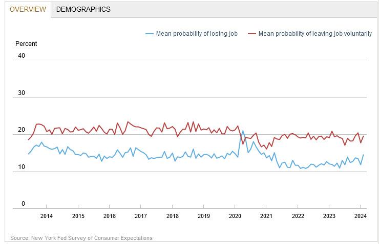
Turning to the labor market, the survey found that the average perceived likelihood of voluntary and involuntary job separations increased, while the perceived likelihood of finding a job (in the event of a job loss) declined. "The mean probability of leaving one’s job voluntarily in the next 12 months also increased, by 1.8 percentage points to 19.5%."
Mean unemployment expectations - or the mean probability that the U.S. unemployment rate will be higher one year from now - decreased by 1.1 percentage points to 36.1%, the lowest reading since February 2022. Additionally, the median one-year-ahead expected earnings growth was unchanged at 2.8%, remaining slightly below its 12-month trailing average of 2.9%.
Turning to household finance, we find the following:
The median expected growth in household income remained unchanged at 3.1%. The series has been moving within a narrow range of 2.9% to 3.3% since January 2023, and remains above the February 2020 pre-pandemic level of 2.7%.
Median household spending growth expectations increased by 0.2 percentage point to 5.2%. The increase was driven by respondents with a high school degree or less.
Median year-ahead expected growth in government debt increased to 9.3% from 8.9%.
The mean perceived probability that the average interest rate on saving accounts will be higher in 12 months increased by 0.6 percentage point to 26.1%, remaining below its 12-month trailing average of 30%.
Perceptions about households’ current financial situations deteriorated somewhat with fewer respondents reporting being better off than a year ago. Year-ahead expectations also deteriorated marginally with a smaller share of respondents expecting to be better off and a slightly larger share of respondents expecting to be worse off a year from now.
The mean perceived probability that U.S. stock prices will be higher 12 months from now increased by 1.4 percentage point to 38.9%.
At the same time, perceptions and expectations about credit access turned less optimistic: "Perceptions of credit access compared to a year ago deteriorated with a larger share of respondents reporting tighter conditions and a smaller share reporting looser conditions compared to a year ago."
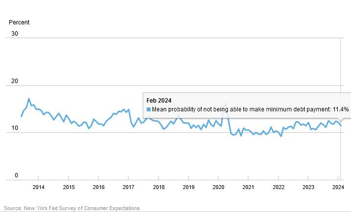
Also, a smaller percentage of consumers, 11.45% vs 12.14% in prior month, expect to not be able to make minimum debt payment over the next three months
Last, and perhaps most humorous, is the now traditional cognitive dissonance one observes with these polls, because at a time when long-term inflation expectations jumped, which clearly suggests that financial conditions will need to be tightened, the number of respondents expecting higher stock prices one year from today jumped to the highest since November 2021... which incidentally is just when the market topped out during the last cycle before suffering a painful bear market.
We use cookies on our website to give you the most relevant experience by remembering your preferences and repeat visits. By clicking “Accept”, you consent to the use of ALL the cookies.
This website uses cookies to improve your experience while you navigate through the website. Out of these, the cookies that are categorized as necessary are stored on your browser as they are essential for the working of basic functionalities of the website. We also use third-party cookies that help us analyze and understand how you use this website. These cookies will be stored in your browser only with your consent. You also have the option to opt-out of these cookies. But opting out of some of these cookies may affect your browsing experience.
Necessary cookies are absolutely essential for the website to function properly. These cookies ensure basic functionalities and security features of the website, anonymously.
Cookie
Duration
Description
cookielawinfo-checbox-analytics
11 months
This cookie is set by GDPR Cookie Consent plugin. The cookie is used to store the user consent for the cookies in the category "Analytics".
cookielawinfo-checbox-functional
11 months
The cookie is set by GDPR cookie consent to record the user consent for the cookies in the category "Functional".
cookielawinfo-checbox-others
11 months
This cookie is set by GDPR Cookie Consent plugin. The cookie is used to store the user consent for the cookies in the category "Other.
cookielawinfo-checkbox-necessary
11 months
This cookie is set by GDPR Cookie Consent plugin. The cookies is used to store the user consent for the cookies in the category "Necessary".
cookielawinfo-checkbox-performance
11 months
This cookie is set by GDPR Cookie Consent plugin. The cookie is used to store the user consent for the cookies in the category "Performance".
viewed_cookie_policy
11 months
The cookie is set by the GDPR Cookie Consent plugin and is used to store whether or not user has consented to the use of cookies. It does not store any personal data.
Functional cookies help to perform certain functionalities like sharing the content of the website on social media platforms, collect feedbacks, and other third-party features.
Performance cookies are used to understand and analyze the key performance indexes of the website which helps in delivering a better user experience for the visitors.
Analytical cookies are used to understand how visitors interact with the website. These cookies help provide information on metrics the number of visitors, bounce rate, traffic source, etc.
Advertisement cookies are used to provide visitors with relevant ads and marketing campaigns. These cookies track visitors across websites and collect information to provide customized ads.


