Uncategorized
Your microbes live on after you die − a microbiologist explains how your necrobiome recycles your body to nourish new life
With the help of the microbes that once played an essential role in keeping you alive, the building blocks of your body go on to become a part of other…
Share this:


Each human body contains a complex community of trillions of microorganisms that are important for your health while you’re alive. These microbial symbionts help you digest food, produce essential vitamins, protect you from infection and serve many other critical functions. In turn, the microbes, which are mostly concentrated in your gut, get to live in a relatively stable, warm environment with a steady supply of food.
But what happens to these symbiotic allies after you die?
As an environmental microbiologist who studies the necrobiome – the microbes that live in, on and around a decomposing body – I’ve been curious about our postmortem microbial legacy. You might assume that your microbes die with you – once your body breaks down and your microbes are flushed into the environment, they won’t survive out in the real world.
In our recently published study, my research team and I share evidence that not only do your microbes continue to live on after you die, they actually play an important role in recycling your body so that new life can flourish.
Microbial life after death
When you die, your heart stops circulating the blood that has carried oxygen throughout your body. Cells deprived of oxygen start digesting themselves in a process called autolysis. Enzymes in those cells – which normally digest carbohydrates, proteins and fats for energy or growth in a controlled way – start to work on the membranes, proteins, DNA and other components that make up the cells.
The products of this cellular breakdown make excellent food for your symbiotic bacteria, and without your immune system to keep them in check and a steady supply of food from your digestive system, they turn to this new source of nutrition.
Gut bacteria, especially a class of microbes called Clostridia, spread through your organs and digest you from the inside out in a process called putrefaction. Without oxygen inside the body, your anaerobic bacteria rely on energy-producing processes that don’t require oxygen, such as fermentation. These create the distinctly odorous-gases signature to decomposition.
From an evolutionary standpoint, it makes sense that your microbes would have evolved ways to adapt to a dying body. Like rats on a sinking ship, your bacteria will soon have to abandon their host and survive out in the world long enough to find a new host to colonize. Taking advantage of the carbon and nutrients of your body allows them to increase their numbers. A bigger population means a higher probability that at least a few will survive out in the harsher environment and successfully find a new body.
A microbial invasion
If you’re buried in the ground, your microbes are flushed into the soil along with a soup of decomposition fluids as your body breaks down. They’re entering an entirely new environment and encountering a whole new microbial community in the soil.
The mixing or coalescence of two distinct microbial communities happens frequently in nature. Coalescence happens when the roots of two plants grow together, when wastewater is emptied into a river or even when two people kiss.
The outcome of mixing – which community dominates and which microbes are active – depends on several factors, such as how much environmental change the microbes experience and who was there first. Your microbes are adapted to the stable, warm environment inside your body where they receive a steady supply of food. In contrast, soil is a particularly harsh place to live – it’s a highly variable environment with steep chemical and physical gradients and big swings in temperature, moisture and nutrients. Furthermore, soil already hosts an exceptionally diverse microbial community full of decomposers that are well adapted to that environment and would presumably outcompete any newcomers.

It’s easy to assume that your microbes will die off once they are outside your body. However, my research team’s previous studies have shown that the DNA signatures of host-associated microbes can be detected in the soil below a decomposing body, on the soil surface and in graves for months or years after the soft tissues of the body have decomposed. This raised the question of whether these microbes are still alive and active or if they are merely in a dormant state waiting for the next host.
Our newest study suggests that your microbes are not only living in the soil but also cooperating with native soil microbes to help decompose your body. In the lab, we showed that mixing soil and decomposition fluids filled with host-associated microbes increased decomposition rates beyond that of the soil communities alone.
We also found that host-associated microbes enhanced nitrogen cycling. Nitrogen is an essential nutrient for life, but most of the nitrogen on Earth is tied up as atmospheric gas that organisms can’t use. Decomposers play a critical role recycling organic forms of nitrogen such as proteins into inorganic forms such as ammonium and nitrate that microbes and plants can use.
Our new findings suggest that our microbes are likely playing a part in this recycling process by converting large nitrogen-containing molecules like proteins and nucleic acids into ammonium. Nitrifying microbes in the soil can then convert the ammonium into nitrate.
Next generation of life
The recycling of nutrients from detritus, or nonliving organic matter, is a core process in all ecosystems. In terrestrial ecosystems, decomposition of dead animals, or carrion, fuels biodiversity and is an important link in food webs.
Living animals are a bottleneck for the carbon and nutrient cycles of an ecosystem. They slowly accumulate nutrients and carbon from large areas of the landscape throughout their lives then deposit it all at once in a small, localized spot when they die. One dead animal can support a whole pop-up food web of microbes, soil fauna and arthropods that make their living off carcasses.
Insect and animal scavengers help further redistribute nutrients in the ecosystem. Decomposer microbes convert the concentrated pools of nutrient-rich organic molecules from our bodies into smaller, more bioavailable forms that other organisms can use to support new life. It’s not uncommon to see plant life flourishing near a decomposing animal, visible evidence that nutrients in bodies are being recycled back into the ecosystem.
That our own microbes play an important role in this cycle is one microscopic way we live on after death.
Jennifer DeBruyn receives funding from the United States Department of Agriculture, National Science Foundation, Department of Justice, and Defense Advanced Research Projects Agency.
link dnaUncategorized
Homes listed for sale in early June sell for $7,700 more
New Zillow research suggests the spring home shopping season may see a second wave this summer if mortgage rates fall
The post Homes listed for sale in…
Share this:

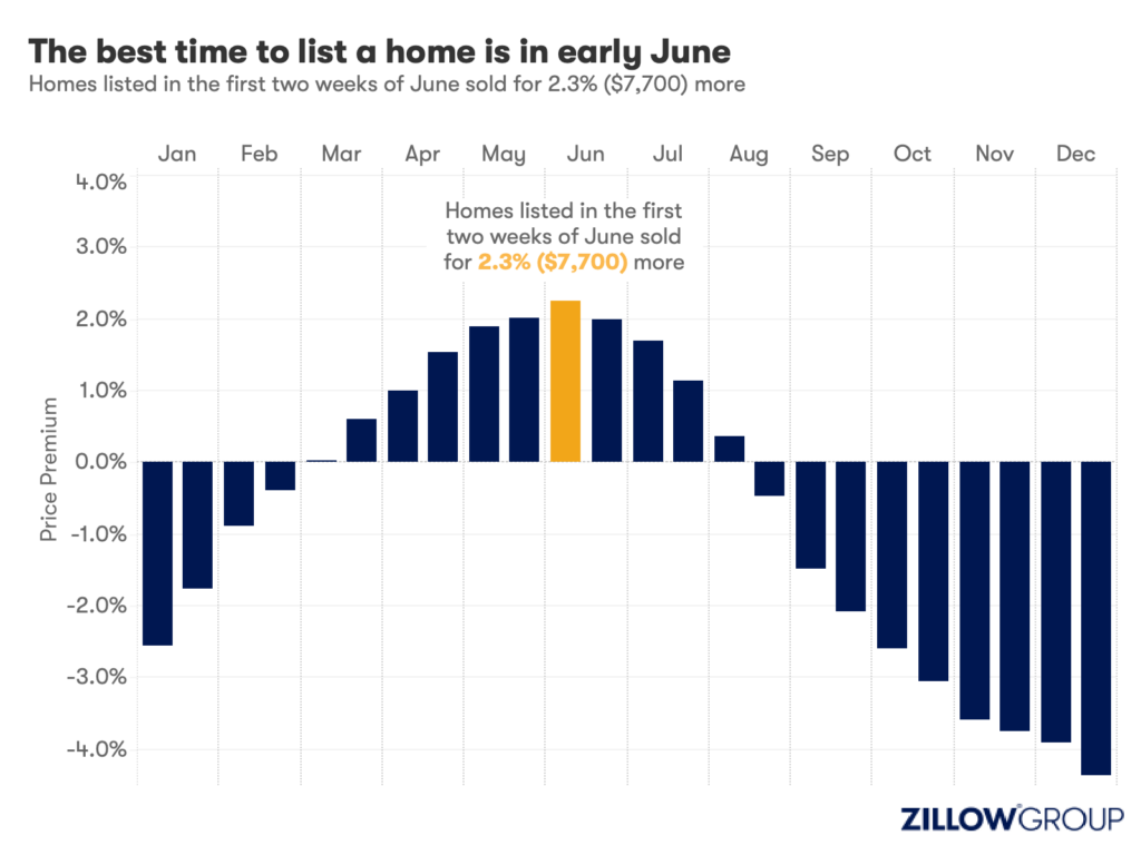
- A Zillow analysis of 2023 home sales finds homes listed in the first two weeks of June sold for 2.3% more.
- The best time to list a home for sale is a month later than it was in 2019, likely driven by mortgage rates.
- The best time to list can be as early as the second half of February in San Francisco, and as late as the first half of July in New York and Philadelphia.
Spring home sellers looking to maximize their sale price may want to wait it out and list their home for sale in the first half of June. A new Zillow® analysis of 2023 sales found that homes listed in the first two weeks of June sold for 2.3% more, a $7,700 boost on a typical U.S. home.
The best time to list consistently had been early May in the years leading up to the pandemic. The shift to June suggests mortgage rates are strongly influencing demand on top of the usual seasonality that brings buyers to the market in the spring. This home-shopping season is poised to follow a similar pattern as that in 2023, with the potential for a second wave if the Federal Reserve lowers interest rates midyear or later.
The 2.3% sale price premium registered last June followed the first spring in more than 15 years with mortgage rates over 6% on a 30-year fixed-rate loan. The high rates put home buyers on the back foot, and as rates continued upward through May, they were still reassessing and less likely to bid boldly. In June, however, rates pulled back a little from 6.79% to 6.67%, which likely presented an opportunity for determined buyers heading into summer. More buyers understood their market position and could afford to transact, boosting competition and sale prices.
The old logic was that sellers could earn a premium by listing in late spring, when search activity hit its peak. Now, with persistently low inventory, mortgage rate fluctuations make their own seasonality. First-time home buyers who are on the edge of qualifying for a home loan may dip in and out of the market, depending on what’s happening with rates. It is almost certain the Federal Reserve will push back any interest-rate cuts to mid-2024 at the earliest. If mortgage rates follow, that could bring another surge of buyers later this year.
Mortgage rates have been impacting affordability and sale prices since they began rising rapidly two years ago. In 2022, sellers nationwide saw the highest sale premium when they listed their home in late March, right before rates barreled past 5% and continued climbing.
Zillow’s research finds the best time to list can vary widely by metropolitan area. In 2023, it was as early as the second half of February in San Francisco, and as late as the first half of July in New York. Thirty of the top 35 largest metro areas saw for-sale listings command the highest sale prices between May and early July last year.
Zillow also found a wide range in the sale price premiums associated with homes listed during those peak periods. At the hottest time of the year in San Jose, homes sold for 5.5% more, a $88,000 boost on a typical home. Meanwhile, homes in San Antonio sold for 1.9% more during that same time period.
| Metropolitan Area | Best Time to List | Price Premium | Dollar Boost |
| United States | First half of June | 2.3% | $7,700 |
| New York, NY | First half of July | 2.4% | $15,500 |
| Los Angeles, CA | First half of May | 4.1% | $39,300 |
| Chicago, IL | First half of June | 2.8% | $8,800 |
| Dallas, TX | First half of June | 2.5% | $9,200 |
| Houston, TX | Second half of April | 2.0% | $6,200 |
| Washington, DC | Second half of June | 2.2% | $12,700 |
| Philadelphia, PA | First half of July | 2.4% | $8,200 |
| Miami, FL | First half of June | 2.3% | $12,900 |
| Atlanta, GA | Second half of June | 2.3% | $8,700 |
| Boston, MA | Second half of May | 3.5% | $23,600 |
| Phoenix, AZ | First half of June | 3.2% | $14,700 |
| San Francisco, CA | Second half of February | 4.2% | $50,300 |
| Riverside, CA | First half of May | 2.7% | $15,600 |
| Detroit, MI | First half of July | 3.3% | $7,900 |
| Seattle, WA | First half of June | 4.3% | $31,500 |
| Minneapolis, MN | Second half of May | 3.7% | $13,400 |
| San Diego, CA | Second half of April | 3.1% | $29,600 |
| Tampa, FL | Second half of June | 2.1% | $8,000 |
| Denver, CO | Second half of May | 2.9% | $16,900 |
| Baltimore, MD | First half of July | 2.2% | $8,200 |
| St. Louis, MO | First half of June | 2.9% | $7,000 |
| Orlando, FL | First half of June | 2.2% | $8,700 |
| Charlotte, NC | Second half of May | 3.0% | $11,000 |
| San Antonio, TX | First half of June | 1.9% | $5,400 |
| Portland, OR | Second half of April | 2.6% | $14,300 |
| Sacramento, CA | First half of June | 3.2% | $17,900 |
| Pittsburgh, PA | Second half of June | 2.3% | $4,700 |
| Cincinnati, OH | Second half of April | 2.7% | $7,500 |
| Austin, TX | Second half of May | 2.8% | $12,600 |
| Las Vegas, NV | First half of June | 3.4% | $14,600 |
| Kansas City, MO | Second half of May | 2.5% | $7,300 |
| Columbus, OH | Second half of June | 3.3% | $10,400 |
| Indianapolis, IN | First half of July | 3.0% | $8,100 |
| Cleveland, OH | First half of July | 3.4% | $7,400 |
| San Jose, CA | First half of June | 5.5% | $88,400 |
The post Homes listed for sale in early June sell for $7,700 more appeared first on Zillow Research.
federal reserve pandemic home sales mortgage rates interest ratesUncategorized
February Employment Situation
By Paul Gomme and Peter Rupert The establishment data from the BLS showed a 275,000 increase in payroll employment for February, outpacing the 230,000…
Share this:

By Paul Gomme and Peter Rupert
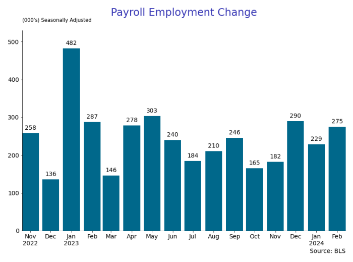
The establishment data from the BLS showed a 275,000 increase in payroll employment for February, outpacing the 230,000 average over the previous 12 months. The payroll data for January and December were revised down by a total of 167,000. The private sector added 223,000 new jobs, the largest gain since May of last year.

Temporary help services employment continues a steep decline after a sharp post-pandemic rise.


Average hours of work increased from 34.2 to 34.3. The increase, along with the 223,000 private employment increase led to a hefty increase in total hours of 5.6% at an annualized rate, also the largest increase since May of last year.

The establishment report, once again, beat “expectations;” the WSJ survey of economists was 198,000. Other than the downward revisions, mentioned above, another bit of negative news was a smallish increase in wage growth, from $34.52 to $34.57.

The household survey shows that the labor force increased 150,000, a drop in employment of 184,000 and an increase in the number of unemployed persons of 334,000. The labor force participation rate held steady at 62.5, the employment to population ratio decreased from 60.2 to 60.1 and the unemployment rate increased from 3.66 to 3.86. Remember that the unemployment rate is the number of unemployed relative to the labor force (the number employed plus the number unemployed). Consequently, the unemployment rate can go up if the number of unemployed rises holding fixed the labor force, or if the labor force shrinks holding the number unemployed unchanged. An increase in the unemployment rate is not necessarily a bad thing: it may reflect a strong labor market drawing “marginally attached” individuals from outside the labor force. Indeed, there was a 96,000 decline in those workers.


Earlier in the week, the BLS announced JOLTS (Job Openings and Labor Turnover Survey) data for January. There isn’t much to report here as the job openings changed little at 8.9 million, the number of hires and total separations were little changed at 5.7 million and 5.3 million, respectively.

As has been the case for the last couple of years, the number of job openings remains higher than the number of unemployed persons.

Also earlier in the week the BLS announced that productivity increased 3.2% in the 4th quarter with output rising 3.5% and hours of work rising 0.3%.

The bottom line is that the labor market continues its surprisingly (to some) strong performance, once again proving stronger than many had expected. This strength makes it difficult to justify any interest rate cuts soon, particularly given the recent inflation spike.
unemployment pandemic unemploymentUncategorized
Mortgage rates fall as labor market normalizes
Jobless claims show an expanding economy. We will only be in a recession once jobless claims exceed 323,000 on a four-week moving average.
Share this:

Everyone was waiting to see if this week’s jobs report would send mortgage rates higher, which is what happened last month. Instead, the 10-year yield had a muted response after the headline number beat estimates, but we have negative job revisions from previous months. The Federal Reserve’s fear of wage growth spiraling out of control hasn’t materialized for over two years now and the unemployment rate ticked up to 3.9%. For now, we can say the labor market isn’t tight anymore, but it’s also not breaking.
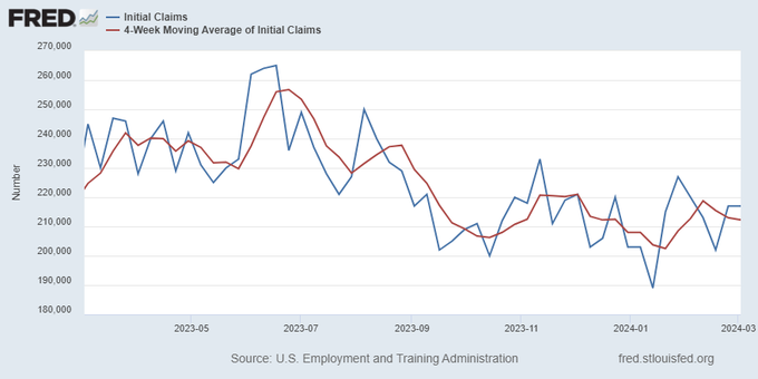
The key labor data line in this expansion is the weekly jobless claims report. Jobless claims show an expanding economy that has not lost jobs yet. We will only be in a recession once jobless claims exceed 323,000 on a four-week moving average.
From the Fed: In the week ended March 2, initial claims for unemployment insurance benefits were flat, at 217,000. The four-week moving average declined slightly by 750, to 212,250
Below is an explanation of how we got here with the labor market, which all started during COVID-19.
1. I wrote the COVID-19 recovery model on April 7, 2020, and retired it on Dec. 9, 2020. By that time, the upfront recovery phase was done, and I needed to model out when we would get the jobs lost back.
2. Early in the labor market recovery, when we saw weaker job reports, I doubled and tripled down on my assertion that job openings would get to 10 million in this recovery. Job openings rose as high as to 12 million and are currently over 9 million. Even with the massive miss on a job report in May 2021, I didn’t waver.
Currently, the jobs openings, quit percentage and hires data are below pre-COVID-19 levels, which means the labor market isn’t as tight as it once was, and this is why the employment cost index has been slowing data to move along the quits percentage.

3. I wrote that we should get back all the jobs lost to COVID-19 by September of 2022. At the time this would be a speedy labor market recovery, and it happened on schedule, too
Total employment data
4. This is the key one for right now: If COVID-19 hadn’t happened, we would have between 157 million and 159 million jobs today, which would have been in line with the job growth rate in February 2020. Today, we are at 157,808,000. This is important because job growth should be cooling down now. We are more in line with where the labor market should be when averaging 140K-165K monthly. So for now, the fact that we aren’t trending between 140K-165K means we still have a bit more recovery kick left before we get down to those levels.

From BLS: Total nonfarm payroll employment rose by 275,000 in February, and the unemployment rate increased to 3.9 percent, the U.S. Bureau of Labor Statistics reported today. Job gains occurred in health care, in government, in food services and drinking places, in social assistance, and in transportation and warehousing.
Here are the jobs that were created and lost in the previous month:

In this jobs report, the unemployment rate for education levels looks like this:
- Less than a high school diploma: 6.1%
- High school graduate and no college: 4.2%
- Some college or associate degree: 3.1%
- Bachelor’s degree or higher: 2.2%

Today’s report has continued the trend of the labor data beating my expectations, only because I am looking for the jobs data to slow down to a level of 140K-165K, which hasn’t happened yet. I wouldn’t categorize the labor market as being tight anymore because of the quits ratio and the hires data in the job openings report. This also shows itself in the employment cost index as well. These are key data lines for the Fed and the reason we are going to see three rate cuts this year.
recession unemployment covid-19 fed federal reserve mortgage rates recession recovery unemployment


-

 Uncategorized3 weeks ago
All Of The Elements Are In Place For An Economic Crisis Of Staggering Proportions
-

 Uncategorized1 month ago
Cathie Wood sells a major tech stock (again)
-

 Uncategorized3 weeks ago
California Counties Could Be Forced To Pay $300 Million To Cover COVID-Era Program
-

 Uncategorized2 weeks ago
Apparel Retailer Express Moving Toward Bankruptcy
-

 Uncategorized4 weeks ago
Industrial Production Decreased 0.1% in January
-

 International3 days ago
Walmart launches clever answer to Target’s new membership program
-

 International3 days ago
EyePoint poaches medical chief from Apellis; Sandoz CFO, longtime BioNTech exec to retire
-

 Uncategorized3 weeks ago
RFK Jr: The Wuhan Cover-Up & The Rise Of The Biowarfare-Industrial Complex